Additive vs Log vs Log-Log Marketing Mix Models#
This notebook compares three MMM specifications available through the link parameter on the MMM class:
Model |
|
Saturation |
Likelihood |
Interpretation |
|---|---|---|---|---|
Additive |
|
|
Normal |
Components add to \(y\) |
Log (multiplicative) |
|
|
LogNormal |
Components multiply \(y\) via \(\exp\) |
Log-log (elasticity) |
|
|
LogNormal |
Coefficients are elasticities |
Mathematical Formulation#
All three models share the same linear predictor:
They differ in how \(\mu\) relates to the observed target \(y\):
1. Additive (Identity Link)#
Each component of \(\mu\) contributes additively to \(y\). This is the standard formulation used in most MMM literature.
2. Log (Multiplicative)#
Equivalently, \(\log(y_{\text{scaled}}) \sim \text{Normal}(\mu, \sigma)\), so \(y \propto \exp(\mu)\). Each additive component in \(\mu\) becomes a multiplicative factor on \(y\):
Use this when the data-generating process is multiplicative (e.g. sales = baseline \(\times\) media uplift \(\times\) seasonality).
3. Log-Log (Elasticity)#
Same as the log model, but the saturation function is \(\beta \log(1 + x)\) (LogSaturation) instead of a sigmoidal curve. The coefficient \(\beta\) has an elasticity-like interpretation: approximately the % change in \(y\) per 1% change in spend.
Use this when channel response follows a power-law / constant-elasticity relationship and you want directly interpretable media coefficients.
Trend Handling#
A raw integer trend \(t = 0, 1, \ldots, n\) behaves differently depending on the link function:
Identity link: \(\gamma_t \cdot t\) adds a linear trend to \(y\).
Log link: \(\gamma_t \cdot t\) in log-space gives exponential growth \(y \propto \exp(\gamma_t \cdot t)\).
With the quickstart’s prior \(\gamma \sim N(0, 0.05)\) and \(t\) up to ~200, the log-space contribution could reach \(\exp(10) \approx 22{,}000\times\), completely degenerate. To avoid this, we normalize the trend to \([0, 1]\) for the log and log-log models, so \(\gamma_t\) directly represents the total multiplicative trend factor via \(\exp(\gamma_t)\).
Prepare Notebook#
import warnings

import arviz as az
import matplotlib.pyplot as plt
import matplotlib.ticker as mtick
import numpy as np
import pandas as pd
from pymc_extras.prior import Prior

from pymc_marketing.mmm import GeometricAdstock, LogisticSaturation, LogSaturation
from pymc_marketing.mmm.mmm import MMM

warnings.filterwarnings("ignore")

az.style.use("arviz-darkgrid")
plt.rcParams["figure.figsize"] = [12, 7]
plt.rcParams["figure.dpi"] = 100

%load_ext autoreload
%autoreload 2
%config InlineBackend.figure_format = "retina"
seed = sum(map(ord, "mmm_multiplicative"))
rng = np.random.default_rng(seed=seed)
Data Loading and Preparation#
We use a synthetic weekly dataset with two media channels (x1, x2), two event indicators, and a sales target. All three models will be fitted to the same data so that any differences in the decomposition reflect the link function choice, not the training set.
url = "https://raw.githubusercontent.com/pymc-labs/pymc-marketing/main/data/mmm_example.csv"
data = pd.read_csv(url, parse_dates=["date_week"])
data.head()
| date_week | y | x1 | x2 | event_1 | event_2 | dayofyear | t | |
|---|---|---|---|---|---|---|---|---|
| 0 | 2018-04-02 | 3984.662237 | 0.318580 | 0.0 | 0.0 | 0.0 | 92 | 0 |
| 1 | 2018-04-09 | 3762.871794 | 0.112388 | 0.0 | 0.0 | 0.0 | 99 | 1 |
| 2 | 2018-04-16 | 4466.967388 | 0.292400 | 0.0 | 0.0 | 0.0 | 106 | 2 |
| 3 | 2018-04-23 | 3864.219373 | 0.071399 | 0.0 | 0.0 | 0.0 | 113 | 3 |
| 4 | 2018-04-30 | 4441.625278 | 0.386745 | 0.0 | 0.0 | 0.0 | 120 | 4 |
# Raw integer trend (for the additive model, matching the quickstart)
data["t"] = range(len(data))

# Normalized trend in [0, 1] (for log/log-log models, avoids exponential blow-up)
data["t_norm"] = data["t"] / data["t"].max()

y = data["y"]

# Two versions of X: one per link type
X_additive = data.drop(columns=["y"])
X_log = data.drop(columns=["y", "t"]).copy()

print(f"Observations: {len(data)}")
print(f"Target range: [{y.min():.1f}, {y.max():.1f}]")
print(f"All y > 0: {(y > 0).all()}  (required for log link)")
Observations: 179
Target range: [3192.9, 8312.4]
All y > 0: True  (required for log link)
CHANNELS = ["x1", "x2"]
CONTROL_COLUMNS_ADDITIVE = ["event_1", "event_2", "t"]
CONTROL_COLUMNS_LOG = ["event_1", "event_2", "t_norm"]
fig, axes = plt.subplots(3, 1, figsize=(12, 9), sharex=True)

# Sales
axes[0].plot(data["date_week"], data["y"], color="black", linewidth=2)
axes[0].set(ylabel="Sales", title="Target Variable: Sales")

# Channel 1
axes[1].plot(data["date_week"], data["x1"], color="C0", linewidth=2)
axes[1].set(ylabel="Spend", title="Channel x1")

# Channel 2
axes[2].plot(data["date_week"], data["x2"], color="C1", linewidth=2)
axes[2].set(xlabel="Date", ylabel="Spend", title="Channel x2");
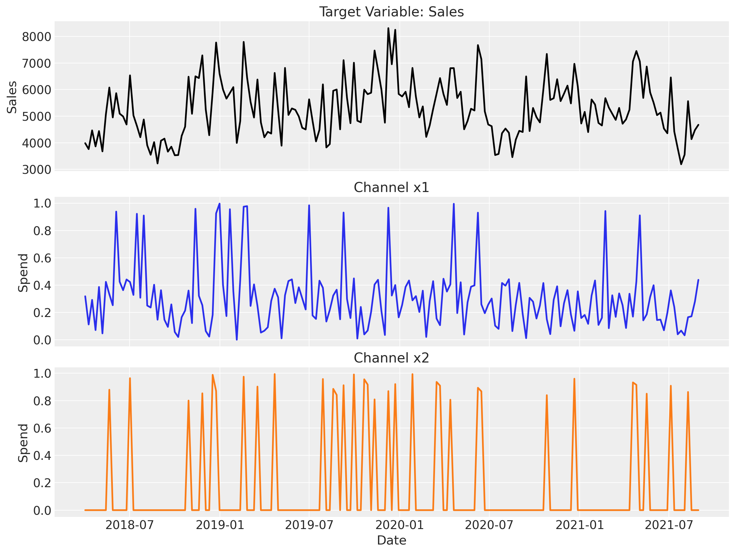
Channel x1 carries the bulk of the spend and shows clear seasonality; x2 is smaller and more sporadic. Sales visually track x1, suggesting it will dominate the estimated media effect. The two event columns (not plotted) are binary indicators for one-off promotions.
Model 1: Additive (Identity Link)#
This is the standard additive MMM from the quickstart notebook. The linear predictor \(\mu\) maps directly to the expected value of \(y\) via the identity link and a Normal likelihood.
# --- Additive model config (from quickstart) ---
additive_model_config = {
    "intercept": Prior("Normal", mu=0.5, sigma=0.2),
    "saturation_beta": Prior("HalfNormal", sigma=prior_sigma, dims="channel"),
    "gamma_control": Prior("Normal", mu=0, sigma=0.05, dims="control"),
    "gamma_fourier": Prior("Laplace", mu=0, b=0.2, dims="fourier_mode"),
    "likelihood": Prior("Normal", sigma=Prior("HalfNormal", sigma=6), dims="date"),
}


mmm_additive = MMM(
    model_config=additive_model_config,
    target_column="y",
    date_column="date_week",
    channel_columns=CHANNELS,
    control_columns=CONTROL_COLUMNS_ADDITIVE,
    yearly_seasonality=2,
    adstock=GeometricAdstock(l_max=8),
    saturation=LogisticSaturation(),
    link="identity",
)

mmm_additive.build_model(X_additive, y)
mmm_additive.add_original_scale_contribution_variable(
    [
        "intercept_contribution",
        "control_contribution",
        "channel_contribution",
        "fourier_contribution",
        "yearly_seasonality_contribution",
        "y",
    ]
)
mmm_additive.table()
                                         Variable  Expression                 Dimensions
──────────────────────────────────────────────────────────────────────────────────────────────────────────
                                  channel_scale =  Data                       channel[2]
                                   target_scale =  Data
                                   channel_data =  Data                       date[179] × channel[2]
                                    target_data =  Data                       date[179]
                                   control_data =  Data                       date[179] × control[3]
                                      dayofyear =  Data                       date[179]

                         intercept_contribution ~  Normal(0.5, 0.2)
                                  adstock_alpha ~  Beta(2, 1, 3)              channel[2]
                                 saturation_lam ~  Gamma(2, 3, f())           channel[2]
                                saturation_beta ~  HalfNormal(0, <constant>)  channel[2]
                                  gamma_control ~  Normal(3, 0, 0.05)         control[3]
                                  gamma_fourier ~  Laplace(4, 0, 0.2)         fourier_mode[4]
                                        y_sigma ~  HalfNormal(0, 6)
                                                                              Parameter count = 15

                           channel_contribution =  f()                        date[179] × channel[2]
                           control_contribution =  f()                        date[179] × control[3]
                           fourier_contribution =  f()                        date[179] × fourier_mode[4]
                yearly_seasonality_contribution =  f()                        date[179]
        total_media_contribution_original_scale =  f()
          intercept_contribution_original_scale =  f()
            control_contribution_original_scale =  f()                        date[179] × control[3]
            channel_contribution_original_scale =  f()                        date[179] × channel[2]
            fourier_contribution_original_scale =  f()                        date[179] × fourier_mode[4]
 yearly_seasonality_contribution_original_scale =  f()                        date[179]
                               y_original_scale =  f()                        date[179]

                                              y ~  Normal(f(), f())           date[179]
fit_kwargs = {
    "chains": 4,
    "target_accept": 0.85,
    "nuts_sampler": "nutpie",
    "random_seed": rng,
}

_ = mmm_additive.fit(X_additive, y, **fit_kwargs)
Sampler Progress
Total Chains: 4
Active Chains: 0
Finished Chains: 4
Sampling for now
Estimated Time to Completion: now
| Progress | Draws | Divergences | Step Size | Gradients/Draw |
|---|---|---|---|---|
| 2000 | 0 | 0.23 | 15 | |
| 2000 | 0 | 0.22 | 63 | |
| 2000 | 0 | 0.24 | 15 | |
| 2000 | 0 | 0.25 | 15 |
Sampling complete. We inspect the trace plots for convergence before interpreting the results.
def plot_trace(mmm, model_name, var_names):
    """Plot trace for key media parameters."""
    _ = az.plot_trace(
        data=mmm.fit_result,
        var_names=var_names,
        compact=True,
        backend_kwargs={"figsize": (10, 2 * len(var_names)), "layout": "constrained"},
    )
    plt.suptitle(
        f"Trace Plot — {model_name}",
        y=1.05,
        fontsize=18,
        fontweight="bold",
    )


TRACE_VAR_NAMES = [
    "saturation_beta",
    "saturation_lam",
    "adstock_alpha",
]

plot_trace(
    mmm_additive,
    model_name="Additive",
    var_names=TRACE_VAR_NAMES,
)

Well-behaved traces show stationary chains that mix well and overlap in their marginal densities. Check the reported number of divergences (ideally zero) before interpreting the posteriors.
def plot_posterior_predictive(mmm, y_obs, model_name):
    y_hat_orig = mmm.idata.posterior["y_original_scale"]
    y_hat_flat = y_hat_orig.stack(sample=("chain", "draw")).values

    fig, ax = plt.subplots()
    dates = mmm.X["date_week"]
    ax.plot(dates, y_obs, color="black", label="observed")
    mean = y_hat_flat.mean(axis=-1)
    ax.plot(dates, mean, color="C0", label="posterior mean")
    for hdi_prob, alpha in zip([0.94, 0.5], [0.15, 0.3], strict=True):
        az.plot_hdi(
            dates,
            y_hat_orig,
            smooth=False,
            hdi_prob=hdi_prob,
            color="C0",
            fill_kwargs={"alpha": alpha, "label": f"{hdi_prob: 0.0%} HDI"},
            ax=ax,
        )
    ax.set(xlabel="date", ylabel="y")
    ax.legend()
    ax.set_title(f"Posterior Predictive — {model_name}", fontsize=18, fontweight="bold")
    return fig, ax


fig, ax = plot_posterior_predictive(mmm_additive, model_name="Additive", y_obs=y)
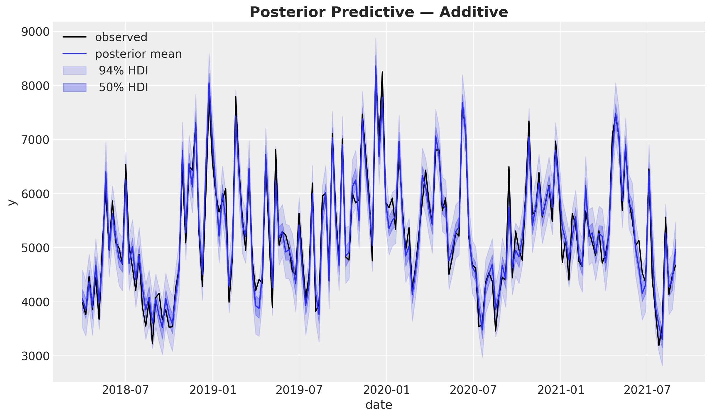
The posterior mean closely tracks the observed data and the HDI bands are reasonably tight, indicating a good in-sample fit. The model captures the seasonal pattern visible in the raw sales data.
Decomposing contributions in the additive model#
compute_mean_contributions_over_time() uses a unified counterfactual decomposition for all link types. Each column answers: “how much would \(\hat y(t)\) decrease if we removed this component?”
For component \(j\) with value \(v_j(t)\) in the linear predictor:
where \(\text{inv}\) is the inverse link and \(s\) = target_scale.
With an identity link \(\text{inv}\) is the identity function, so this simplifies to:
The resulting columns sum exactly to \(\hat y(t)\) at every date. Each line in the decomposition plot below can be read as “this many units of \(y\) came from this component on this date.”
contributions_additive = mmm_additive.compute_mean_contributions_over_time()
contributions_additive.head()
| date | x1 | x2 | event_1 | event_2 | t | yearly_seasonality | intercept | |
|---|---|---|---|---|---|---|---|---|
| 0 | 2018-04-02 | 1081.310948 | 0.0 | 0.0 | 0.0 | 0.000000 | 21.605785 | 2950.875124 |
| 1 | 2018-04-09 | 830.860562 | 0.0 | 0.0 | 0.0 | 5.130659 | 73.587865 | 2950.875124 |
| 2 | 2018-04-16 | 1291.052197 | 0.0 | 0.0 | 0.0 | 10.261317 | 119.363314 | 2950.875124 |
| 3 | 2018-04-23 | 789.377086 | 0.0 | 0.0 | 0.0 | 15.391976 | 153.622369 | 2950.875124 |
| 4 | 2018-04-30 | 1537.007585 | 0.0 | 0.0 | 0.0 | 20.522635 | 171.787010 | 2950.875124 |
def plot_decomposition(contributions_df, model_name, date_col="date"):
    """Plot component contributions over time (line plot, handles mixed signs)."""
    component_cols = [c for c in contributions_df.columns if c != date_col]
    fig, ax = plt.subplots(figsize=(12, 7))
    for col in component_cols:
        ax.plot(
            contributions_df[date_col], contributions_df[col], linewidth=1.5, label=col
        )
    ax.set(
        xlabel="date",
        ylabel="contribution (original scale)",
    )
    ax.set_title(
        f"Decomposition (Posterior Mean) — {model_name}", fontsize=18, fontweight="bold"
    )
    ax.legend(loc="center left", bbox_to_anchor=(1, 0.5))
    return fig, ax


fig, ax = plot_decomposition(contributions_additive, "Additive")
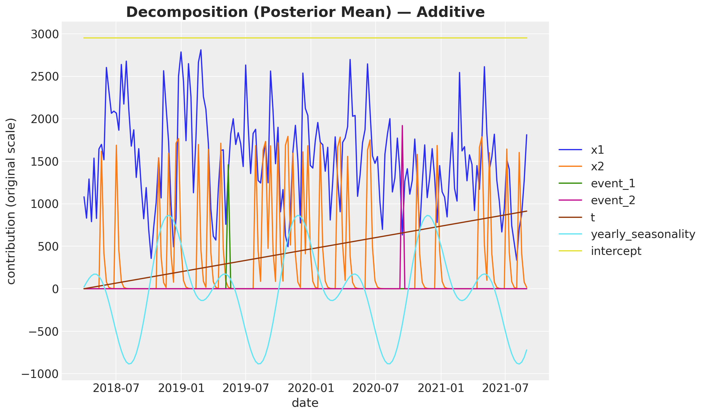
The line plot shows each component’s time-varying contribution in original-scale units.
In many cases, we are not just interested in the posterior mean decomposition, but the entire distribution of contributions. We can also extract this fromt the model:
contributions_additive_posterior = (
    mmm_additive.compute_counterfactual_contributions_dataset()
)

contributions_additive_posterior
<xarray.Dataset> Size: 34MB
Dimensions:             (chain: 4, draw: 1000, date: 179)
Coordinates:
  * chain               (chain) int64 32B 0 1 2 3
  * draw                (draw) int64 8kB 0 1 2 3 4 5 ... 994 995 996 997 998 999
  * date                (date) datetime64[ns] 1kB 2018-04-02 ... 2021-08-30
Data variables:
    x1                  (chain, draw, date) float64 6MB 1.062e+03 ... 2.009e+03
    x2                  (chain, draw, date) float64 6MB 0.0 0.0 ... 76.81 15.97
    event_1             (chain, draw, date) float64 6MB 0.0 0.0 0.0 ... 0.0 0.0
    event_2             (chain, draw, date) float64 6MB 0.0 0.0 0.0 ... 0.0 0.0
    t                   (chain, draw, date) float64 6MB 0.0 4.695 ... 978.7
    yearly_seasonality  (chain, draw, date) float64 6MB 49.09 87.61 ... -710.1
intercept (chain, draw) float64 32kB 2.995e+03 ... 2.841e+03fig, ax = plt.subplots()
az.plot_hdi(
contributions_additive_posterior["date"],
contributions_additive_posterior["x1"],
hdi_prob=0.94,
color="C0",
smooth=False,
fill_kwargs={"alpha": 0.5, "label": r"$x_1$ (94% HDI)"},
ax=ax,
)
az.plot_hdi(
contributions_additive_posterior["date"],
contributions_additive_posterior["x2"],
hdi_prob=0.94,
color="C1",
smooth=False,
fill_kwargs={"alpha": 0.5, "label": r"$x_2$ (94% HDI)"},
ax=ax,
)
ax.legend(loc="upper right")
ax.set(xlabel="date", ylabel="contribution (original scale)")
ax.set_title(
"Counterfactual Contributions (HDI) - Additive Model",
fontsize=18,
fontweight="bold",
);
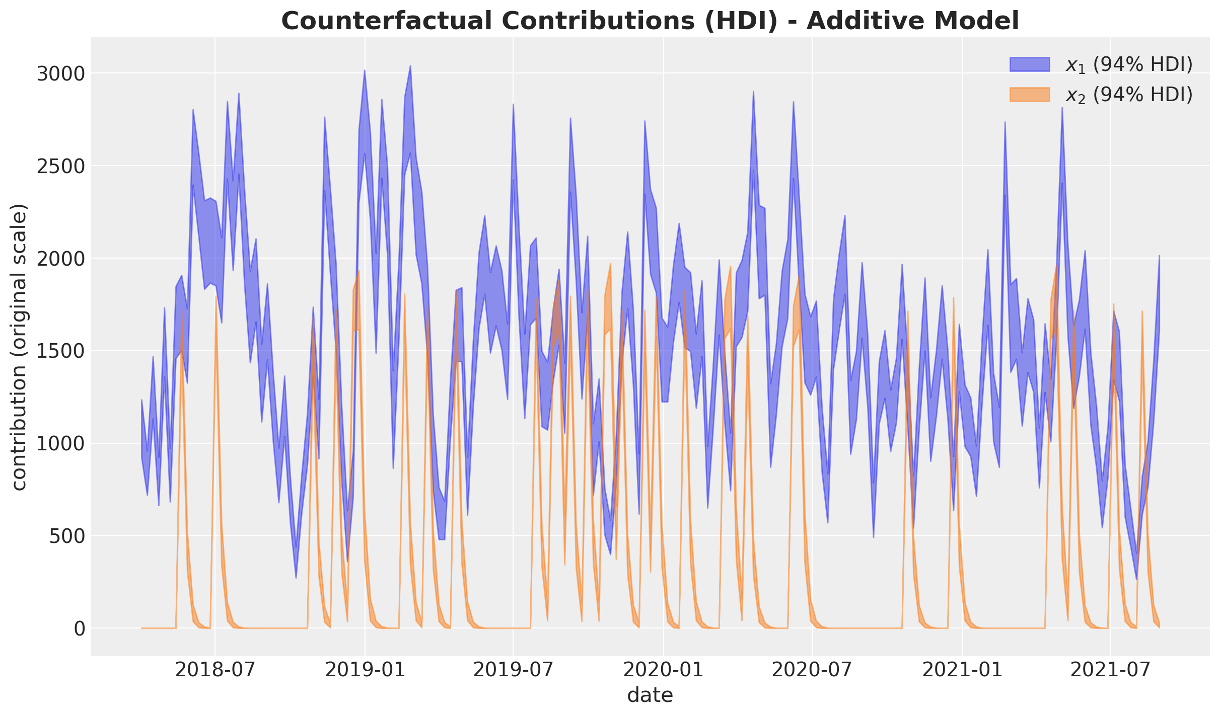
To summarize the relative importance of the two media channels we can look at their posterior share distributions below.
fig, ax = mmm_additive.plot.channel_contribution_share_hdi(figsize=(9, 5))
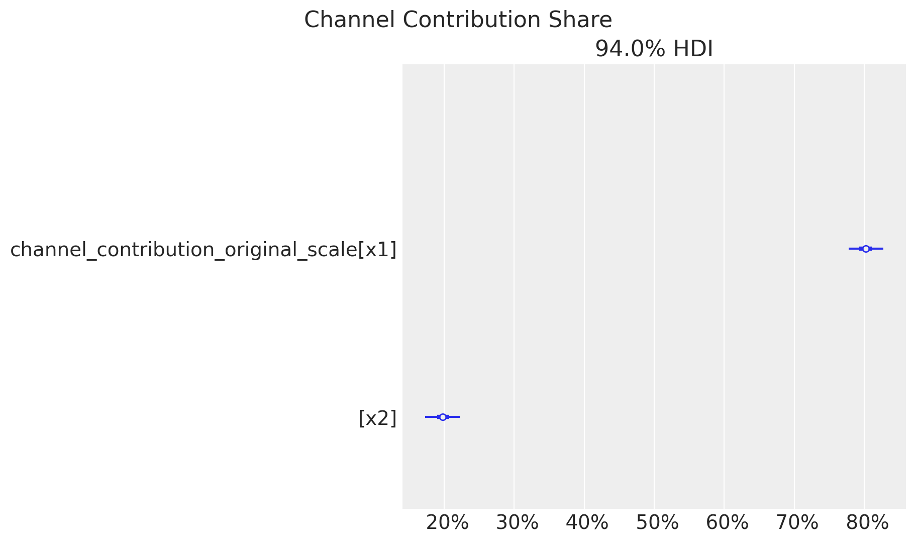
Channel x1 captures the majority of the estimated media effect, consistent with its higher spend volume. The posterior distributions are well separated, giving confidence that the model can distinguish the two channels.
Model 2: Log (Multiplicative)#
With link="log", the linear predictor \(\mu\) is the same additive combination, but each component becomes a multiplicative factor on \(y\) via \(\exp(\cdot)\):
The likelihood is LogNormal, so \(\log(y_{\text{scaled}}) \sim N(\mu, \sigma)\).
Note on trend: We use t_norm (normalized to \([0, 1]\)) instead of the raw integer t to avoid exponential blow-up. The coefficient \(\gamma_t\) now represents the total log-scale trend over the observation period, and \(\exp(\gamma_t)\) is the multiplicative factor from start to end.
# --- Log / log-log model config ---
# The link="log" defaults handle intercept (Normal(0, 5)) and likelihood
# (LogNormal(sigma=HalfNormal(0.5))). We override saturation_beta,
# gamma_control (wider for [0,1]-scaled trend), and gamma_fourier.
log_model_config = {
    "saturation_beta": Prior("HalfNormal", sigma=prior_sigma, dims="channel"),
    "gamma_control": Prior("Normal", mu=0, sigma=0.5, dims="control"),
    "gamma_fourier": Prior("Laplace", mu=0, b=0.2, dims="fourier_mode"),
}

mmm_log = MMM(
    model_config=log_model_config,
    target_column="y",
    date_column="date_week",
    channel_columns=CHANNELS,
    control_columns=CONTROL_COLUMNS_LOG,
    yearly_seasonality=2,
    adstock=GeometricAdstock(l_max=8),
    saturation=LogisticSaturation(),
    link="log",
)

mmm_log.build_model(X_log, y)
mmm_log.table()
                                  Variable  Expression                 Dimensions
───────────────────────────────────────────────────────────────────────────────────────────────────
                           channel_scale =  Data                       channel[2]
                            target_scale =  Data
                            channel_data =  Data                       date[179] × channel[2]
                             target_data =  Data                       date[179]
                            control_data =  Data                       date[179] × control[3]
                               dayofyear =  Data                       date[179]

                  intercept_contribution ~  Normal(0, 5)
                           adstock_alpha ~  Beta(2, 1, 3)              channel[2]
                          saturation_lam ~  Gamma(2, 3, f())           channel[2]
                         saturation_beta ~  HalfNormal(0, <constant>)  channel[2]
                           gamma_control ~  Normal(3, 0, 0.5)          control[3]
                           gamma_fourier ~  Laplace(4, 0, 0.2)         fourier_mode[4]
                                 y_sigma ~  HalfNormal(0, 0.5)
                                                                       Parameter count = 15

                    channel_contribution =  f()                        date[179] × channel[2]
                    control_contribution =  f()                        date[179] × control[3]
                    fourier_contribution =  f()                        date[179] × fourier_mode[4]
         yearly_seasonality_contribution =  f()                        date[179]
                                      mu =  f()                        date[179]
 total_media_contribution_original_scale =  f()
                        y_original_scale =  f()                        date[179]

                                       y ~  LogNormal(mu, f())         date[179]
_ = mmm_log.fit(X=X_log, y=y, **fit_kwargs)
Sampler Progress
Total Chains: 4
Active Chains: 0
Finished Chains: 4
Sampling for now
Estimated Time to Completion: now
| Progress | Draws | Divergences | Step Size | Gradients/Draw |
|---|---|---|---|---|
| 2000 | 0 | 0.27 | 15 | |
| 2000 | 0 | 0.27 | 31 | |
| 2000 | 0 | 0.27 | 15 | |
| 2000 | 0 | 0.28 | 15 |
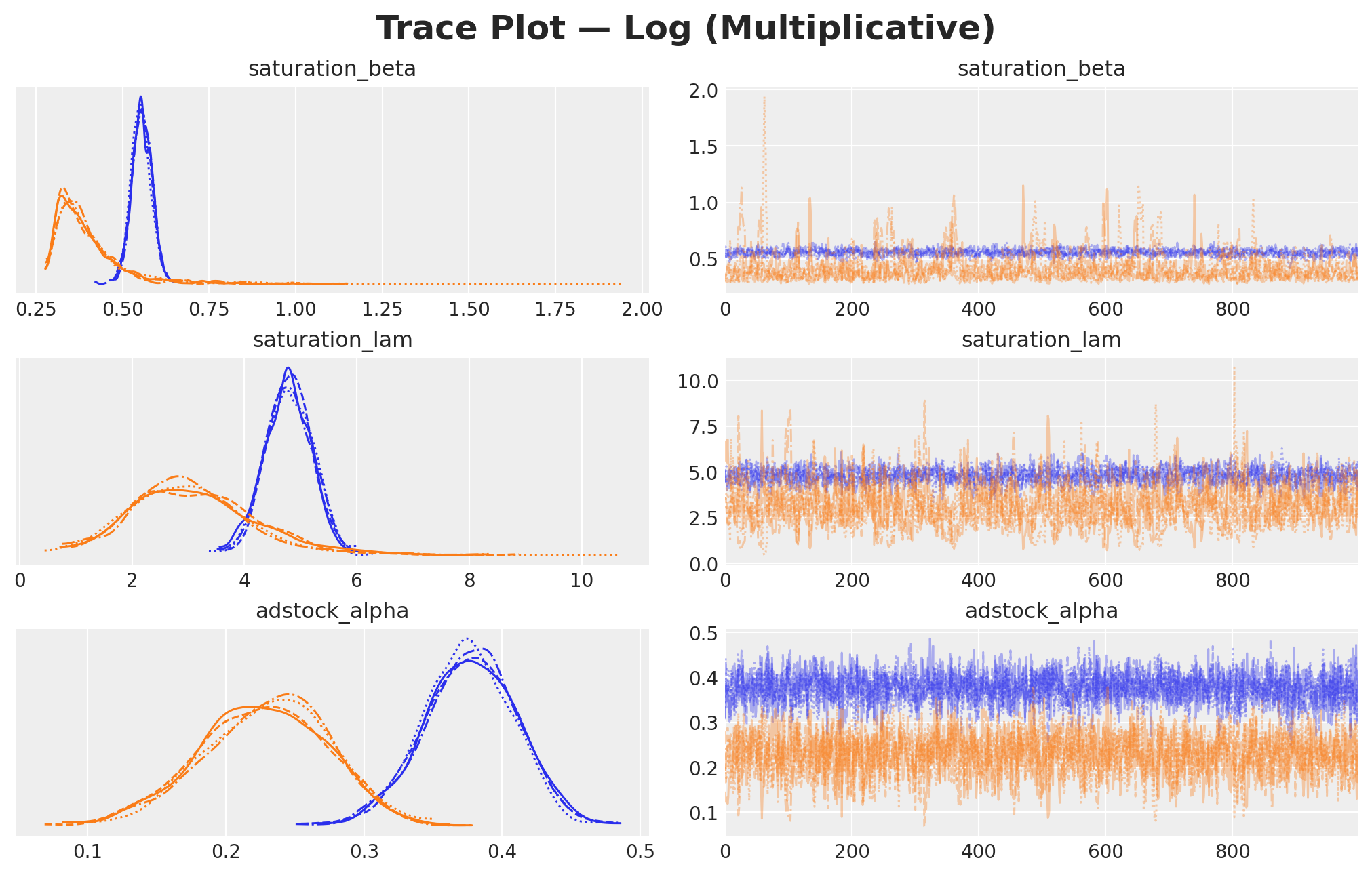
Sampling complete. We check traces and divergences before proceeding.
plot_trace(
    mmm_log,
    model_name="Log (Multiplicative)",
    var_names=TRACE_VAR_NAMES,
)
fig, ax = plot_posterior_predictive(mmm_log, model_name="Log (Multiplicative)", y_obs=y)
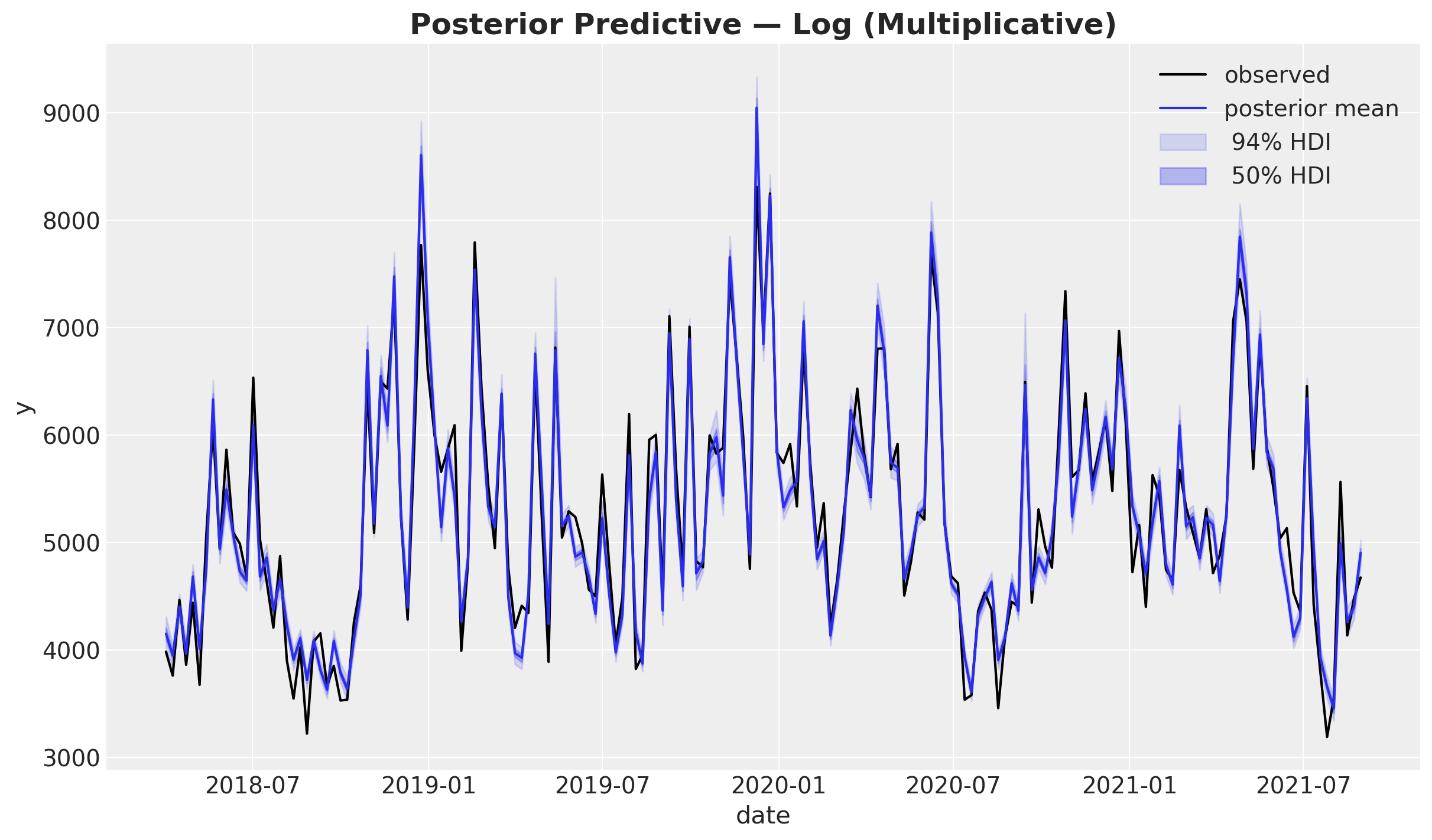
The log model’s posterior predictive fit is comparable to the additive model. Because the data was generated additively, both specifications can approximate it well — the log-link simply re-expresses the same pattern through an exponential transformation.
Decomposing contributions in a multiplicative model#
The business question: “How much of my weekly sales came from TV, from search, from seasonality, from baseline demand?”
For the additive model each term already answered this in the same units as sales. For a log-link model the components multiply each other’s effects (they are exponents inside exp(·)), so no single component has a direct dollar interpretation on its own.
compute_mean_contributions_over_time() uses the same unified counterfactual decomposition as for the additive model. For each component \(j\) with log-space value \(v_j(t)\):
Business reading: each column answers “if we removed this component entirely, how much would predicted sales drop?” — a genuine counterfactual question.
Why columns do not sum to \(\hat y(t)\)
In a multiplicative model, components interact: removing channel A reduces the multiplicative base that channel B amplifies, and vice versa. Each component’s counterfactual captures its own effect plus its share of every interaction it participates in. When you add all per-component counterfactuals together, the shared interactions are counted more than once, so the sum exceeds \(\hat y(t)\).
This is an inherent property of per-component counterfactuals in any non-linear model and is not a defect. It simply means you cannot stack these contributions into an exact partition of \(\hat y(t)\). Instead, interpret each component on its own terms: “removing X would cost us this much.”
contributions_log = mmm_log.compute_mean_contributions_over_time()
contributions_log.head()
| date | x1 | x2 | event_1 | event_2 | t_norm | yearly_seasonality | intercept | |
|---|---|---|---|---|---|---|---|---|
| 0 | 2018-04-02 | 903.428186 | 0.0 | 0.0 | 0.0 | 0.000000 | 37.456809 | -6571.248326 |
| 1 | 2018-04-09 | 666.445597 | 0.0 | 0.0 | 0.0 | 3.902770 | 73.549817 | -6251.853366 |
| 2 | 2018-04-16 | 1090.541638 | 0.0 | 0.0 | 0.0 | 8.701475 | 118.781532 | -6973.960380 |
| 3 | 2018-04-23 | 625.650738 | 0.0 | 0.0 | 0.0 | 11.742525 | 131.254959 | -6275.988969 |
| 4 | 2018-04-30 | 1330.397229 | 0.0 | 0.0 | 0.0 | 18.484885 | 169.574619 | -7414.978742 |
How to read the decomposition plot#
Each line shows one component’s counterfactual contribution in original-scale units (the same units as \(y\) — e.g. dollars, revenue, conversions). It answers: “if we removed this component, how much would predicted sales decrease?”
Media channels (x1, x2): the incremental sales lift from each channel. These fluctuate with spend patterns and are typically non-negative. They answer “how many extra sales did this channel drive each week?”
Controls (events, trend): the dollar impact of external factors. Event contributions spike on event dates; trend captures the long-run direction.
Seasonality: the cyclic pattern in sales attributed to time-of-year effects.
Why the intercept looks different from the additive model
In an additive model the intercept represents a fixed baseline level of sales — it is flat over time and always positive.
In a multiplicative (log-link) model the intercept plays a fundamentally different role. It is a scaling factor \(e^{\alpha}\) that, together with all other multiplicative components, produces the observed sales. If the combined media, control, and seasonality effects already push the prediction above the observed level, the intercept compensates by becoming negative in log-space (\(\alpha < 0\)), acting as a dampening factor (\(e^{\alpha} < 1\)).
The counterfactual question “what if we removed the intercept?” therefore has a counter-intuitive answer: removing a dampening factor would increase predicted sales, which is why the intercept contribution can be negative in the plot. Its temporal variation comes from the fact that the counterfactual scales with total predicted sales — approximately:
When \(\hat y(t)\) is high the dampening effect is large in absolute terms, so the intercept line mirrors the shape of total sales (including seasonality and media spikes), just flipped and scaled.
This is not a modeling defect. It reflects the algebraic reality that in a multiplicative model no single component can be interpreted as “baseline sales” in isolation. The intercept is best understood as the residual scaling factor that reconciles all other components with the observed data.
The non-summing property
Unlike the additive model, summing all lines at a given date will give a total greater than \(\hat y(t)\). This is expected: in a multiplicative model each component amplifies the others, and those shared interaction effects are counted in every component’s counterfactual. Think of it as overlapping credit rather than a partitioning error. Each component’s value is individually correct — “removing X costs us this much” — even though the values cannot be stacked into an exact pie chart of \(\hat y(t)\).
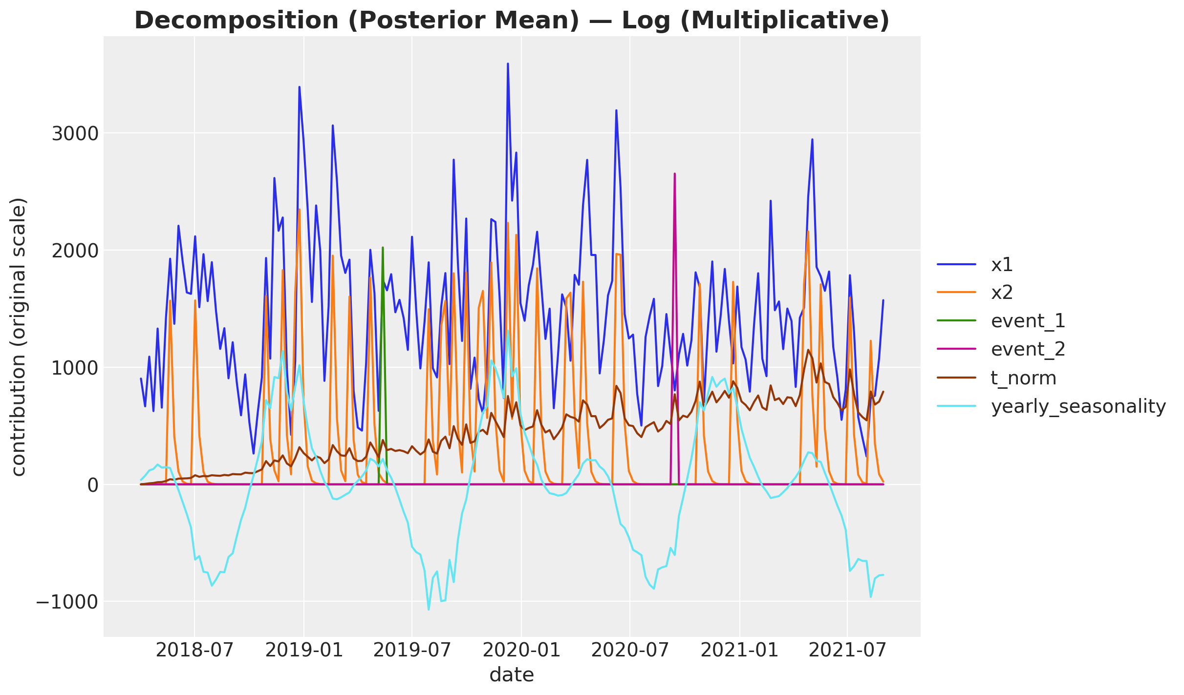
plot_decomposition(contributions_log, model_name="Log (Multiplicative)")
(<Figure size 1200x700 with 1 Axes>,
 <Axes: title={'center': 'Decomposition (Posterior Mean) — Log (Multiplicative)'}, xlabel='date', ylabel='contribution (original scale)'>)
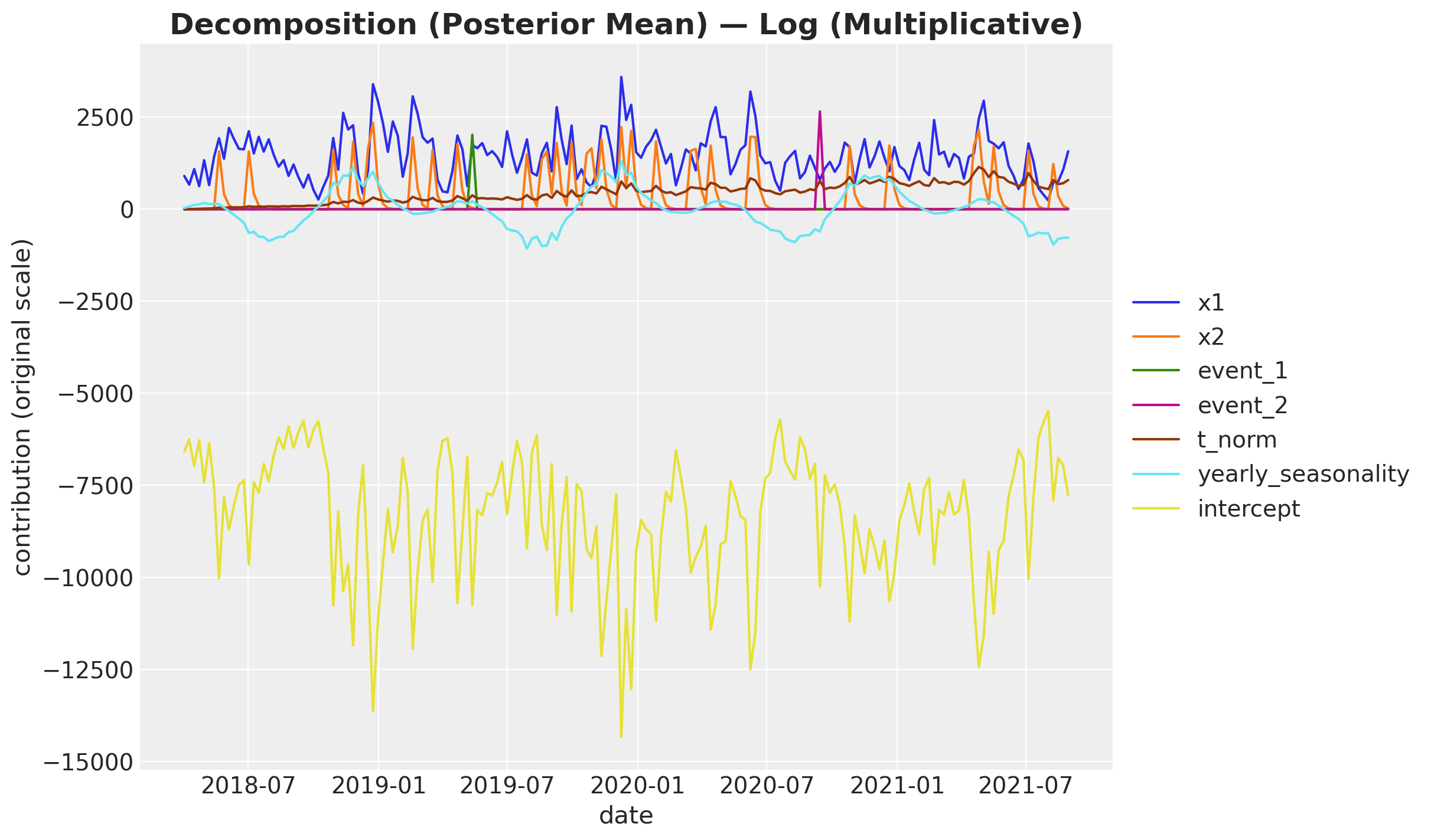
The intercept’s large dampening contribution dominates the y-axis and compresses the other lines. Dropping it makes the channel and control contributions easier to compare.
plot_decomposition(
    contributions_log.drop(columns=["intercept"]), model_name="Log (Multiplicative)"
)
(<Figure size 1200x700 with 1 Axes>,
 <Axes: title={'center': 'Decomposition (Posterior Mean) — Log (Multiplicative)'}, xlabel='date', ylabel='contribution (original scale)'>)
This plot looks much closer to the additive model’s decomposition.
Model 3: Log-Log (Elasticity)#
The log-log model combines link="log" with LogSaturation, which applies \(\beta \log(1 + x)\) instead of a sigmoidal curve. This gives the model a
constant-elasticity structure:
The coefficient \(\beta_c\) approximates the elasticity: the percentage change in \(y\) for a 1% change in spend on channel \(c\). This is directly interpretable for marketing decision-making.
Note: Under the default scaling pipeline, channel data is divided by channel_scale, so these are approximate elasticities with respect to scaled spend rather than strict textbook elasticities.
mmm_loglog = MMM(
    model_config=log_model_config,
    target_column="y",
    date_column="date_week",
    channel_columns=CHANNELS,
    control_columns=CONTROL_COLUMNS_LOG,
    yearly_seasonality=2,
    adstock=GeometricAdstock(l_max=8),
    saturation=LogSaturation(),
    link="log",
)
mmm_loglog.build_model(X_log, y)
mmm_loglog.add_original_scale_contribution_variable(
    [
        "intercept_contribution",
        "control_contribution",
        "channel_contribution",
        "fourier_contribution",
        "yearly_seasonality_contribution",
        "y",
    ]
)
mmm_loglog.table()
                                         Variable  Expression                 Dimensions
──────────────────────────────────────────────────────────────────────────────────────────────────────────
                                  channel_scale =  Data                       channel[2]
                                   target_scale =  Data
                                   channel_data =  Data                       date[179] × channel[2]
                                    target_data =  Data                       date[179]
                                   control_data =  Data                       date[179] × control[3]
                                      dayofyear =  Data                       date[179]

                         intercept_contribution ~  Normal(0, 5)
                                  adstock_alpha ~  Beta(2, 1, 3)              channel[2]
                                saturation_beta ~  HalfNormal(0, <constant>)  channel[2]
                                  gamma_control ~  Normal(3, 0, 0.5)          control[3]
                                  gamma_fourier ~  Laplace(4, 0, 0.2)         fourier_mode[4]
                                        y_sigma ~  HalfNormal(0, 0.5)
                                                                              Parameter count = 13

                           channel_contribution =  f()                        date[179] × channel[2]
                           control_contribution =  f()                        date[179] × control[3]
                           fourier_contribution =  f()                        date[179] × fourier_mode[4]
                yearly_seasonality_contribution =  f()                        date[179]
                                             mu =  f()                        date[179]
        total_media_contribution_original_scale =  f()
                               y_original_scale =  f()                        date[179]
          intercept_contribution_original_scale =  f()
            control_contribution_original_scale =  f()                        date[179] × control[3]
            channel_contribution_original_scale =  f()                        date[179] × channel[2]
            fourier_contribution_original_scale =  f()                        date[179] × fourier_mode[4]
 yearly_seasonality_contribution_original_scale =  f()                        date[179]

                                              y ~  LogNormal(mu, f())         date[179]
_ = mmm_loglog.fit(
    X=X_log,
    y=y,
    chains=4,
    target_accept=0.85,
    nuts_sampler="nutpie",
    random_seed=rng,
)
Sampler Progress
Total Chains: 4
Active Chains: 0
Finished Chains: 4
Sampling for now
Estimated Time to Completion: now
| Progress | Draws | Divergences | Step Size | Gradients/Draw |
|---|---|---|---|---|
| 2000 | 0 | 0.45 | 15 | |
| 2000 | 0 | 0.37 | 7 | |
| 2000 | 0 | 0.42 | 7 | |
| 2000 | 0 | 0.40 | 31 |
Sampling complete. We check traces and divergences before proceeding.
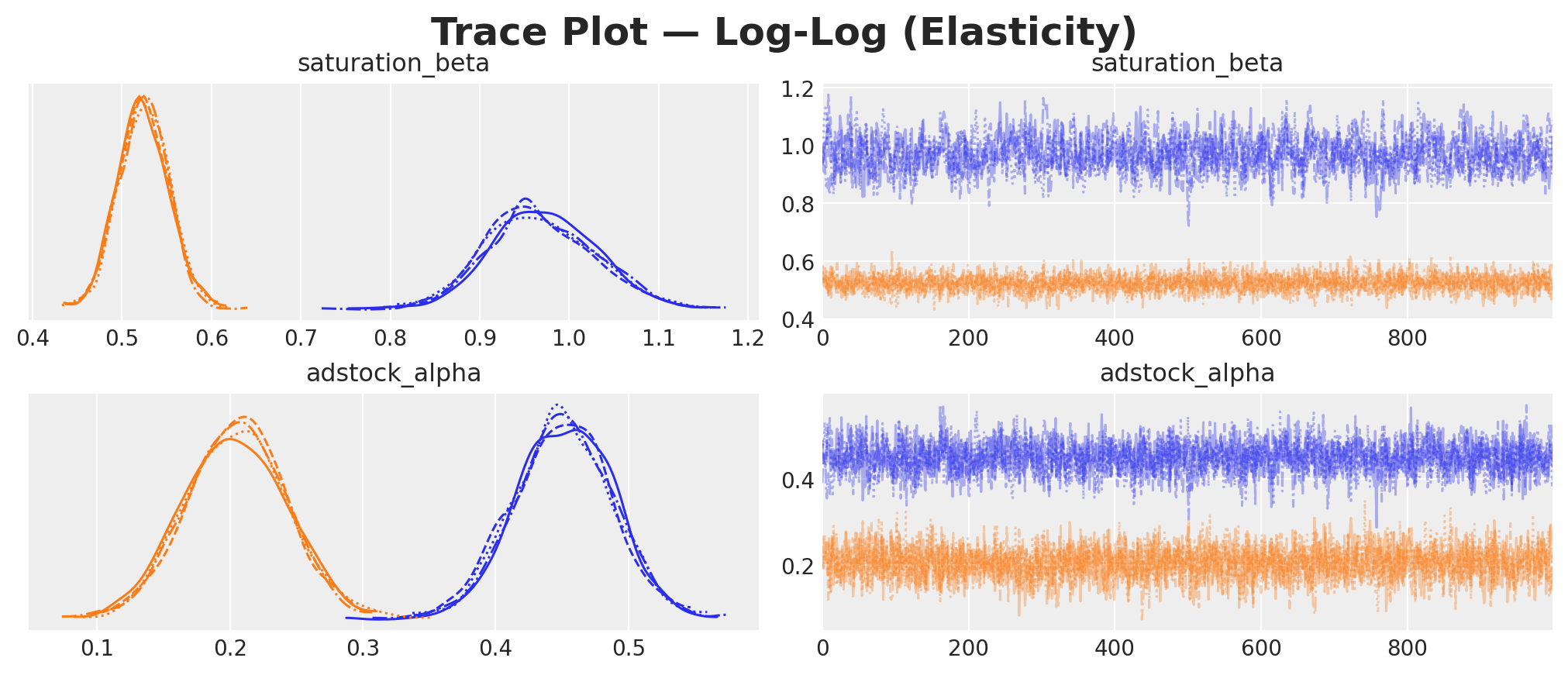
plot_trace(
    mmm_loglog, "Log-Log (Elasticity)", var_names=["saturation_beta", "adstock_alpha"]
)
fig, ax = plot_posterior_predictive(
    mmm_loglog, model_name="Log-Log (Elasticity)", y_obs=y
)
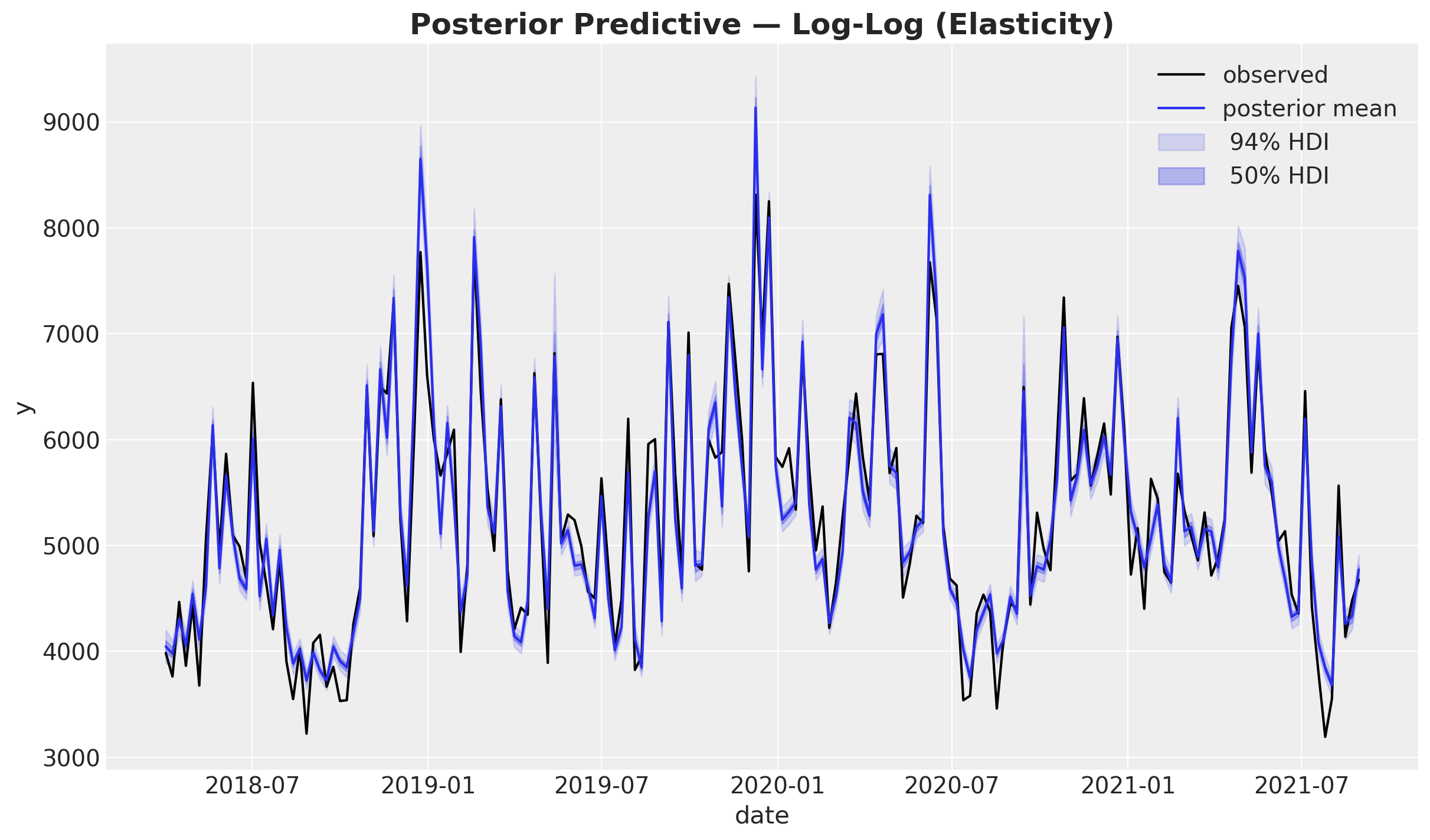
The log-log model fits the data comparably to the other two specifications. On this synthetic additive dataset the three models converge on similar predictions, though their internal decompositions differ.
contributions_loglog = mmm_loglog.compute_mean_contributions_over_time()
contributions_loglog.head()
| date | x1 | x2 | event_1 | event_2 | t_norm | yearly_seasonality | intercept | |
|---|---|---|---|---|---|---|---|---|
| 0 | 2018-04-02 | 586.131824 | 0.0 | 0.0 | 0.0 | 0.000000 | 41.395140 | -5776.179551 |
| 1 | 2018-04-09 | 476.318674 | 0.0 | 0.0 | 0.0 | 4.266044 | 83.935657 | -5680.206182 |
| 2 | 2018-04-16 | 767.139992 | 0.0 | 0.0 | 0.0 | 9.233000 | 131.522347 | -6150.039165 |
| 3 | 2018-04-23 | 484.853799 | 0.0 | 0.0 | 0.0 | 13.030373 | 152.242630 | -5789.421142 |
| 4 | 2018-04-30 | 957.038345 | 0.0 | 0.0 | 0.0 | 19.464421 | 187.706453 | -6489.430840 |
The counterfactual decomposition for the log-log model works identically to the log model — same formula, same non-summing property. The only difference is the saturation function shape (LogSaturation instead of LogisticSaturation), which affects how much each channel contributes, not how contributions are computed.
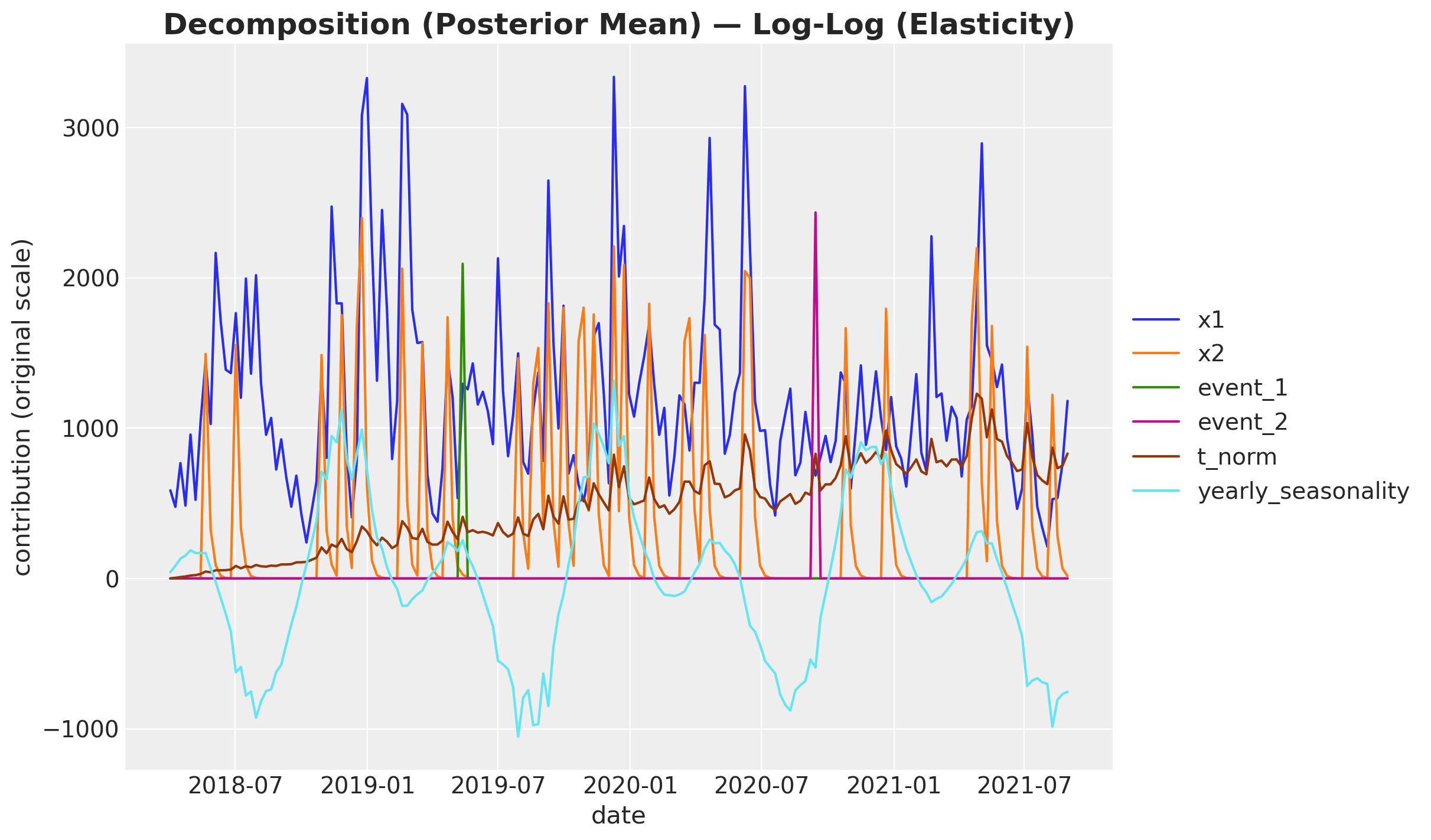
fig, ax = plot_decomposition(contributions_loglog, "Log-Log (Elasticity)")
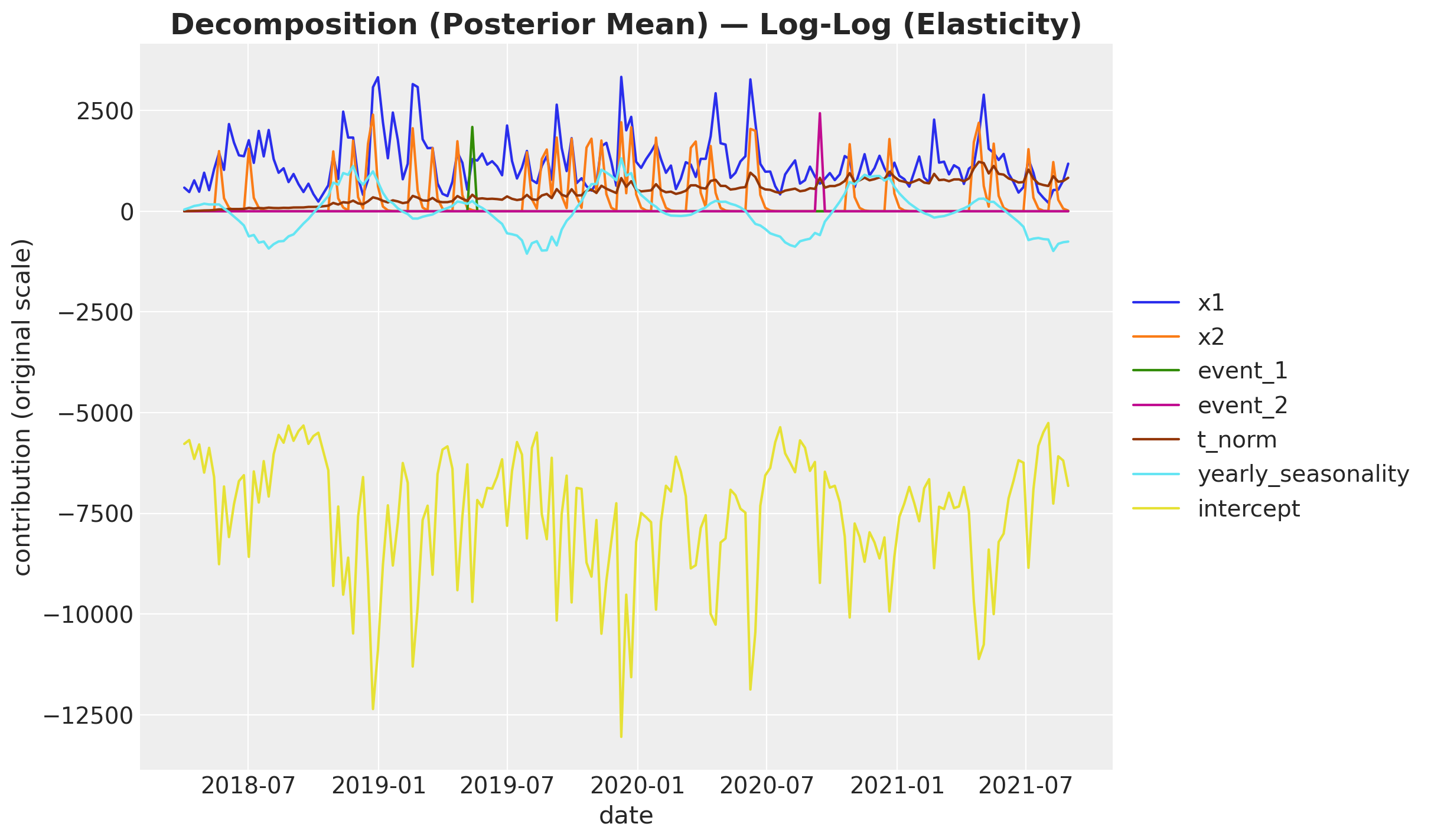
As with the log model, dropping the intercept makes the remaining contributions easier to read.
fig, ax = plot_decomposition(
    contributions_loglog.drop(columns=["intercept"]), "Log-Log (Elasticity)"
)
Decomposition Comparison#
Having fitted all three models to the same data, we now compare their decompositions side by side. Since this synthetic dataset was generated with an additive process, the additive model should recover the true contributions most faithfully. The multiplicative models re-express the same fit through a different lens — the goal here is to see where they agree and where the link function choice matters.
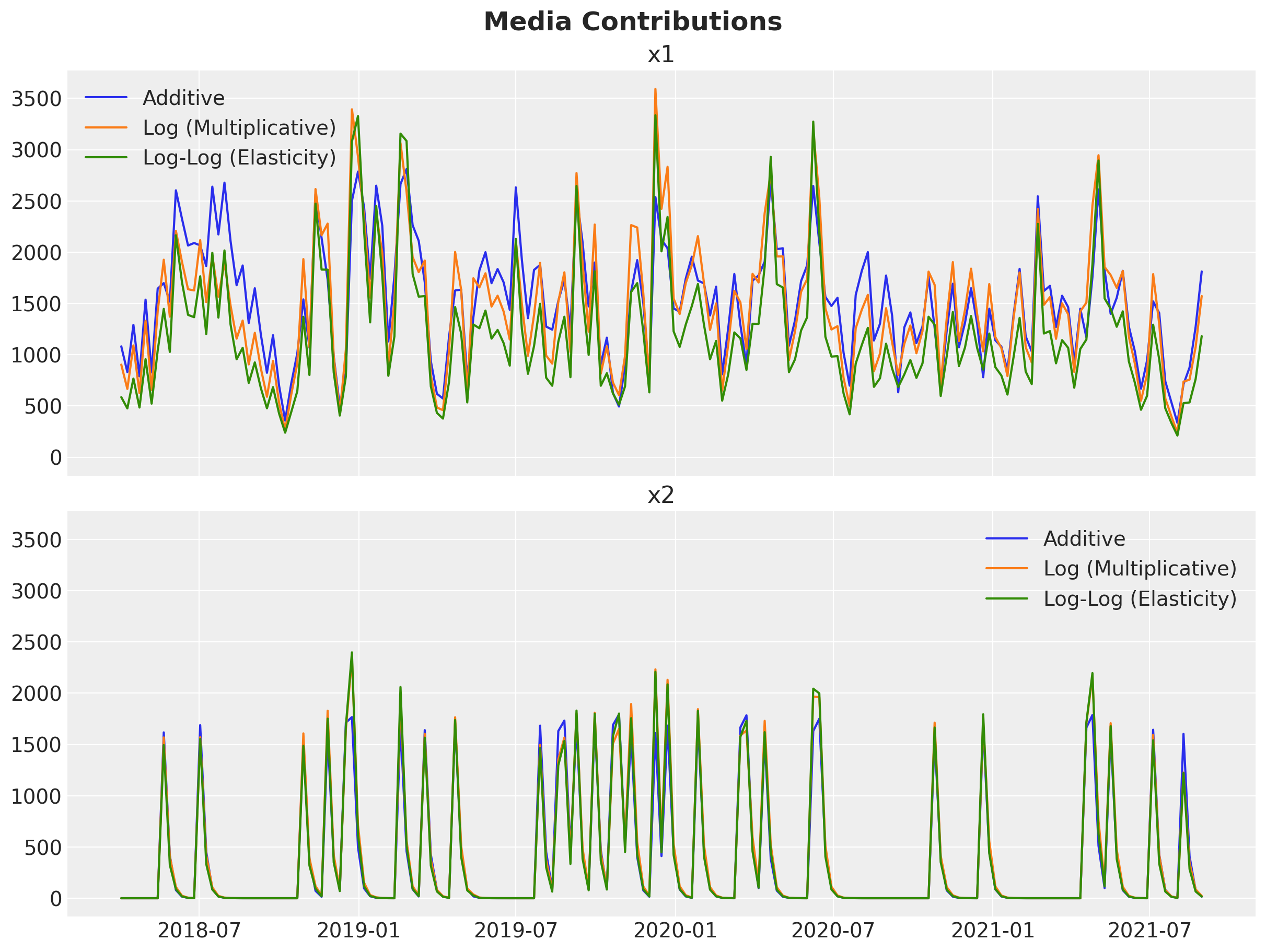
Media Contributions#
The time-series overlay below shows whether the three models agree on the shape of each channel’s contribution over time. The bar chart that follows compares their relative magnitude (which channel gets more credit).
decomp_data = [
    ("Additive", contributions_additive),
    ("Log (Multiplicative)", contributions_log),
    ("Log-Log (Elasticity)", contributions_loglog),
]
fig, ax = plt.subplots(
    nrows=len(CHANNELS),
    ncols=1,
    figsize=(12, 9),
    sharex=True,
    sharey=True,
    layout="constrained",
)

for name, df in decomp_data:
    ax[0].plot(df["date"], df["x1"], label=name)
    ax[1].plot(df["date"], df["x2"], label=name)

ax[0].legend()
ax[0].set_title("x1")
ax[1].legend()
ax[1].set_title("x2")

fig.suptitle("Media Contributions", fontsize=18, fontweight="bold");
fig, axes = plt.subplots(
    nrows=1,
    ncols=3,
    figsize=(12, 5),
    sharex=True,
    sharey=True,
    layout="constrained",
)
for ax, (name, df) in zip(axes, decomp_data, strict=True):
    channel_total = df[CHANNELS].sum()
    channel_share = channel_total / channel_total.sum()
    channel_share.plot.bar(ax=ax, color=["C0", "C1"])
    ax.set(title=name, xlabel="", ylabel="channel share" if ax == axes[0] else "")
    ax.yaxis.set_major_formatter(mtick.PercentFormatter(xmax=1.0))

fig.suptitle("Channel Contribution Shares", fontsize=18, fontweight="bold");
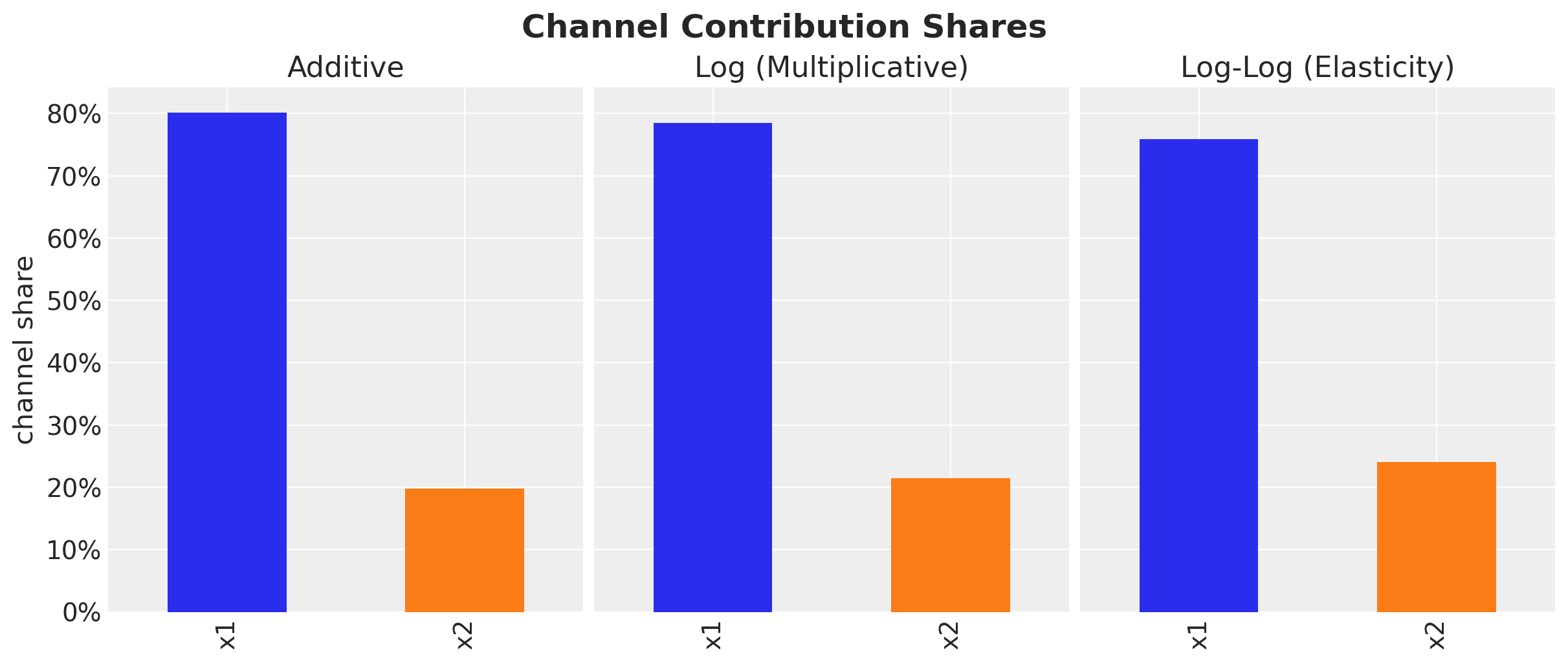
All three models agree on relative channel importance: x1 consistently receives the larger share. This is reassuring, even though the multiplicative models decompose the total differently, they reach the same directional conclusion about which channel drives more sales.
Non-Media Contributions#
We compare how events and seasonality are attributed across models. Because these components represent shared structure (not marketing decision levers), agreement here increases confidence that the media estimates are not absorbing unrelated variation.
fig, ax = plt.subplots(
    nrows=3,
    ncols=1,
    figsize=(12, 9),
    sharex=True,
    sharey=True,
    layout="constrained",
)

for name, df in decomp_data:
    ax[0].plot(df["date"], df["event_1"], label=name)
    ax[1].plot(df["date"], df["event_2"], label=name)
    ax[2].plot(df["date"], df["yearly_seasonality"], label=name)

ax[0].legend()
ax[0].set_title("event_1")
ax[1].legend()
ax[1].set_title("event_2")
ax[2].legend()
ax[2].set_title("yearly_seasonality")

fig.suptitle("None-Media Contributions", fontsize=18, fontweight="bold");
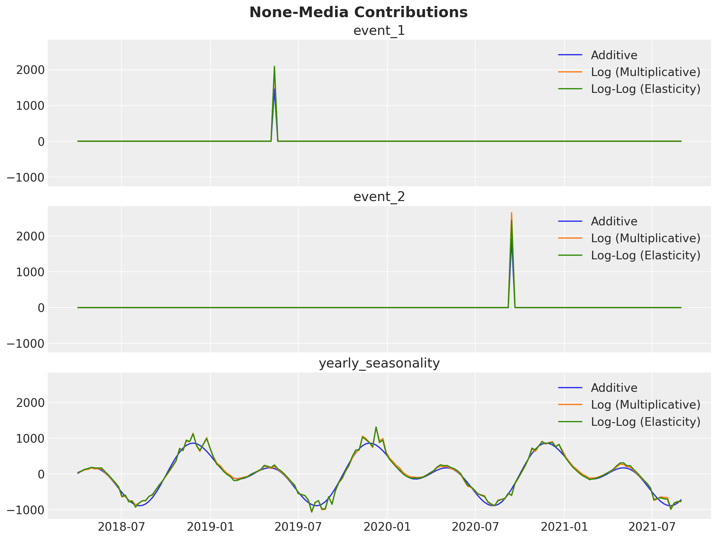
Events and seasonality contributions are broadly consistent across models, with only minor differences in amplitude. This suggests the three specifications agree on the non-media structure and differ mainly in how they partition the remaining media effect.
Summary Metrics#
We close with a quick quantitative comparison. MAE and RMSE measure in-sample prediction error in the original units of \(y\); MAPE expresses the same error as a percentage of observed sales. Divergences indicate sampling problems — ideally zero for all models.
y_hat_additive = (
    mmm_additive.idata["posterior"]["y_original_scale"]
    .mean(dim=("chain", "draw"))
    .to_numpy()
)
y_hat_log = (
    mmm_log.idata["posterior"]["y_original_scale"]
    .mean(dim=("chain", "draw"))
    .to_numpy()
)
y_hat_loglog = (
    mmm_loglog.idata["posterior"]["y_original_scale"]
    .mean(dim=("chain", "draw"))
    .to_numpy()
)

results = []
for name, mmm_obj, y_hat in [
    ("Additive", mmm_additive, y_hat_additive),
    ("Log (Multiplicative)", mmm_log, y_hat_log),
    ("Log-Log (Elasticity)", mmm_loglog, y_hat_loglog),
]:
    n_div = mmm_obj.idata["sample_stats"]["diverging"].sum().item()
    residuals = y.values - y_hat
    mae = np.abs(residuals).mean()
    rmse = np.sqrt((residuals**2).mean())
    mape = np.abs(residuals / y.values).mean() * 100

    results.append(
        {
            "Model": name,
            "Divergences": int(n_div),
            "MAE": round(mae, 2),
            "RMSE": round(rmse, 2),
            "MAPE (%)": round(mape, 2),
        }
    )

summary_df = pd.DataFrame(results)
print(summary_df.to_string(index=False))
               Model  Divergences    MAE   RMSE  MAPE (%)
            Additive            0 196.25 248.45      3.89
Log (Multiplicative)            0 207.60 264.40      4.05
Log-Log (Elasticity)            0 236.05 303.93      4.59
On this dataset, the additive model achieves the lowest prediction error across all metrics. This is expected: the synthetic data was generated by an additive process, so the additive model has a structural advantage.
This result should not be taken as evidence that the additive model is universally preferable. On real-world data the true generating process is unknown, and multiplicative relationships (e.g. media amplifying a seasonal baseline) are common. The choice of link function should be guided by:
Domain knowledge: does the business context suggest additive or multiplicative effects?
Data characteristics: are sales strictly positive? Is variance proportional to the mean (favoring log-link)?
Model diagnostics: convergence, posterior predictive checks, and out-of-sample performance.
When in doubt, fitting multiple specifications (as done here) and comparing diagnostics is a practical strategy.
%load_ext watermark
%watermark -n -u -v -iv -w -p pymc_marketing,pymc,nutpie
Last updated: Thu, 07 May 2026

Python implementation: CPython
Python version       : 3.13.12
IPython version      : 9.11.0

pymc_marketing: 0.19.2
pymc          : 5.28.1
nutpie        : 0.16.8

arviz         : 0.23.4
matplotlib    : 3.10.8
numpy         : 2.4.2
pandas        : 2.3.3
pymc_extras   : 0.9.3
pymc_marketing: 0.19.2

Watermark: 2.6.0